Ryangineer

Noteworthy Machine Learning Algorithms

  Machine Learning   ⇒   software able to detect patterns, make decisions, predict outcomes, learn from mistakes & optimize own performance without being explicitly programmed to do so

Supervised Learning

Learning a function that maps to an output based on the example of input-output pairs. In other words, training a model on data where the outcome is known, for subsequent application to data where the outcome is not known."
"Present labeled examples to learn from. For instance, when we want to be able to predict the selling price of a house in advance in a real estate market, we can get the historical prices of houses and have a supervised learning algorithm successfully figure out how to associate the prices to the house characteristics.
Using the uppercase letter X we intend to use matrix notation, since we can also treat the y as a response vector (technically a column vector) and the X as a matrix containing all values of the feature vectors, each arranged into a separate column of the matrix. . . . building a function that can answer the question about how X can imply y . . . [with] a functional mapping that can translate X values into y without error or with an acceptable margin of error. . . . to determinate a function of the following kind:" (Massaron, pg 24)

• Active Learning

  Semi-supervised learning algorithm where the software picks examples of data that are most useful to its learning & ignoring the bulk of data in data warehouses or data lakes.

• Online Learning

  In a fast-paced environment, a learning algorithm may stream data as it becomes available, continuously adapting to any new associations between predictive variables & the response.

• Matrix Notation Function

  "When the function is specified, and we have in mind a certain algorithm with certain parameters & an X matrix made up of certain data, conventionally we can refer to it as a hypothesis."

  $y \; =\; h\left(X\right)$
    ↳ where:
    X = a matrix of size (n, p)
    y = a response vector of size n
    n = # of observations
    p = # of variables

  Store the predictive variables (features or attributes) in the X matrix, size n x p:

  $X \; =\; \left[\begin{array}{cccc}{x}_{\mathrm{1,1}}& x_{\mathrm{1,2}}& \mathrm{-}& x_{\mathrm{1,}}{\mathrm{}}_p\\ x_2& x_{\mathrm{2,2}}& \mathrm{-}& x_{\mathrm{2,}}{\mathrm{}}_p\\ \mathrm{.}& \mathrm{.}& \mathrm{-}& \mathrm{.}\\ \mathrm{.}& \mathrm{.}& \mathrm{-}& \mathrm{.}\\ \mathrm{.}& \mathrm{.}& \mathrm{-}& \mathrm{.}\\ x_n{\mathrm{}}_{\mathrm{,1}}& x_n{\mathrm{}}_{\mathrm{,2}}& \mathrm{-}& x_n{\mathrm{}}_{\mathrm{,}}{\mathrm{}}_p\end{array}\right]$

• Linear Regression | Predict Real Values

  Estimate or predict real values based on continuous variables -> establish relationship between independent variables (matrix of features) & dependent variable (output) by fitting a best line

• Homoscedasticity

  "Homoskedastic . . . refers to a condition in which the variance of the residual, or error term, [that is, the “noise” or random disturbance in the relationship between the independent variables and the dependent variable], in a regression model is constant. That is, the error term does not vary much as the value of the predictor variable changes." Investopedia

• Multicollinearity

  "[R]efers to predictors that are correlated [, that is, highly linearly related,] with other predictors. Multicollinearity occurs when your model includes multiple factors that are correlated not just to your response variable, but also to each other. In other words, it results when you have factors that are a bit redundant." Minitab

• No Free Lunch Theorems (NFL)

  "[S]tate that any one algorithm that searches for an optimal cost or fitness solution is not universally superior to any other algorithm. . . . 'If an algorithm performs better than random search on some class of problems then in must perform worse than random search on the remaining problems.'” Medium

• Parsimonious Model

  "Parsimonious models are simple models [with the least assumptions & variables but] with great explanatory predictive power. They explain data with a minimum number of parameters, or predictor variables. The idea behind parsimonious models stems from Occam's razor, or 'the law of briefness' (sometimes called lex parsimoniae in Latin)." Statistics How To

• Law of Large Numbers

  As the # of experiments grows, so increases the likelihood that the average of their results will reporesent the true value of the population.

• Linear Combination

  A sum where each addendum value is modified by a weight (the coefficients), and, therefore, a smarter form of summation.

• Family of Linear Models or Generalized Linear Model (GLM)

  Function that specifies the relationship between the X, the predictors, & the y, the target, is a linear combination of the X values. By means of special link functions proper transformation of the answer variable, proper constraints on the weights & different optimization procedures (the learning procedures), GLM can solve a very wide range of problems.

• Probability Density Function (PDF)

  A function describing the probability of values in the distribution. For a normal distribution:

  $f\left(x\right|\mu ,\sigma ) \; =\; \frac{1}{\sigma \sqrt{2\pi }}{e}^{-}{\mathrm{}}^{\frac{(x-\mu ){\mathrm{}}^2}{2{\sigma }^2}}$

  • Moments of the PDF

    • First moment: expected value or a generalization of the weighted average, the arithmetic mean

    • Second central moment: variance or expectation of the squared deviation of a random variable

    • Third standardized moment: skewness or a measure of the asymmetry of the probability distribution of a real-valued random variable about its mean

    • Fourth standardized moment: kurtosis or a measure of the "tailedness" of the probability distribution of a real-valued random variable

• Covariation vs. Correlation

  Covariation is a measure of association that is affected by the scale of the variables & is not standardized. When a variable is standardized, it returns a value between -1 to 1, -1 being negatively correlated (one grows, the other shrinks), 1 being positively correlated (one grows, so does the other) & 0 meaning there is no relationship, at all.
  Correlation is a measure of the strength of linear association between two variables, of how close to a straight line your points are.

  • Covariance Expression

    $cov(x_i,y) \; =\; \frac{1}{n} \; *\; \Sigma (x_i \; -\; {\mathrm{x̄}}_i) \; *\; (y \; -\; ȳ)$

  • Pearson's Correlation

    $r \; =\; \frac{1}{n} \; *\; \frac{\Sigma (x_i \; -\; {\mathrm{x̄}}_i) \; *\; (y \; -\; ȳ)}{{\sigma }_{x_i} \; *\; {\sigma }_y}$

• Ordinary Least Squares (OLS)

  Another way to refer to linear regression. "A type of linear least squares method for estimating the unknown parameters in a linear regression model. OLS chooses the parameters of a linear function of a set of explanatory variables by the principle of least squares: minimizing the sum of the squares of the differences between the observed dependent variable (values of the variable being observed) in the given dataset and those predicted by the linear function of the independent variable. Geometrically, this is seen as the sum of the squared distances, parallel to the axis of the dependent variable, between each data point in the set and the corresponding point on the regression surface—the smaller the differences, the better the model fits the data." Wikipedia

• Bias

  The point at which a regression line crosses the y-axis; that is, the predicted value when X = 0.

  bias = y-intercept

• Derivation of Line of Best Fit | Residual Sum of Squares(RSS)

  Linear regression tries to fit a line through a given set of points, choosing the best fit. The best fit is the line that minimizes the summed squared difference between the value dictated by the line for a certain value of x and its corresponding y values. It is optimizing the squared error.

  RSS = Σ(y - ŷ)² → min

• Residuals or Errors

  The difference between the observed values of the dependent variable (y) & the predicted (fitted) values (ŷ).
  "The deviations of the actual y from the predicted y. When forming a linear regression, the predicted Y follows a linear relationship. Deviations from this line, are called residuals; they measure the distance between the actual Y for each N and the line (predicted Y). For a good linear model, the residuals should be small and random. If they are really large it shows the model is not very accurate, and if there is a pattern then it would suggest a non-linear model would fit better for example." r/AskStatistics

  • Each data point has to residuals.
  • Both the sum & the mean of the residuals are equal to zero.
  • If the points in a residual plot are randomly dispersed arount the horizontal axis, the linear regression model is appropriate. Otherwise, a non-linear model is more appropriate.
  • Positive residual ⇒ better than expected predicted value.
  • Negative residual ⇒ less than expected predicted value.
  • Zero residual ⇒ meets the expected value.
  • Residual Sum of Squares ⇒ used to measure the amount of variance in a dataset not explained by the model.
  • Standard Error of Residuals ⇒ the smaller, the more accurate the predictions are.

• Fitted Values or Predicted Values

  The estimates Ŷ_i obtained from a regression line, the predictions.

• Interpolation & Extrapolation

  Interpolation: A linear regresssion model can always work within the range of values from which it learned. Extrapolation: But can provide correct values for its learning boundaries only in certain conditions.

• Kurtosis

  This is a measure of the shape of the distribution of the residuals. A bell-shaped distribution has a zero measure. A negative value points to a too flat distribution; a positive one has too great a peak.
  "A measure of the 'tailedness' of the probability distribution of a real-valued random variable." Wikipedia

  $\mathrm{Kurt} \; =\; \frac{{\mu }_4}{{\sigma }^4}$

• Simple Linear Regression

  Combining one variable in an equation to predict a single outcome

  y = b₀ + b₁x₁
     or
  y = βx + β₀
     or
  y = mx + b
     or
  y = a + bx
     or
  Y_i = b₀ + b₁X_i + e_i
    ↳ where:
    y = response, dependent, criterion, target, outcome, label
    a, b, b₀, β₀ = constant, y-intercept, bias
    m, b, b₁, β = slope, coefficient, gradient, angular coefficient
    x, x₁, X_i = independent, explanatory, predictor variable, matrix of predictors, feature vector, control variable
    e_i = explicit error term
   
  $a \; =\; \frac{\left(\mathrm{\Sigma }y\right)\left(\mathrm{\Sigma }{x}^2\right) \; -\; \left(\mathrm{\Sigma }x\right)\left(\mathrm{\Sigma }xy\right)}{n\left(\mathrm{\Sigma }{x}^2\right) \; -\; \left(\mathrm{\Sigma }x\right){\mathrm{}}^2}$
  $b \; =\; \frac{n\left(\mathrm{\Sigma }xy\right) \; -\; \left(\mathrm{\Sigma }x\right)\left(\mathrm{\Sigma }y\right)}{n\left(\mathrm{\Sigma }{x}^2\right) \; -\; \left(\mathrm{\Sigma }x\right){\mathrm{}}^2}$
  ${\mathrm{b}}_1 \; =\; \frac{\mathrm{\Delta Y}}{\mathrm{\Delta X}}$
  ${\mathrm{ê}}_i \; =\; Y_i \; +\; {\mathrm{Ŷ}}_i$

• Minimization of the Cost Function

  "The search for a line's equation that it is able to minimize the sum of the squared errors of the difference between the line's y values and the original ones." WGU MSDA
  Methods of minimization include Pseudoinverse, QR factorization, & gradient descent.

  • Regression Function of h(X):

    $y \; \approx \; h\left(X\right) \; =\; \beta X \; +\; {\beta }_0$
    Cost function minimized as follows:
    $\frac{1}{2\mathrm{N/mi>}} \; *\; \Sigma \left(h\right(X) \; -\; y){\mathrm{}}^2$

  • Pseudoinverse

    An analytical formula for solving a regression analysis and getting a vector of coefficients out of data, minimizing the cost function:

    $w \; =\; \left(X^{T}X\right){\mathrm{}}^{-1}{X}^{T}y$
    Or solve for w in linear equations called normal equations:
    $\left(X^{T}X\right){\mathrm{}}^{-1} \; *\; w \; =\; X^{T}y$

• Gradient Descent

  "Explaining it simply, it resembles walking blind in the mountains. If you want to descend to the lowest valley, even if you don't know and can't see the path, you can proceed approximately by going downhill for a while, then stopping, then going downhill again and so on, always aiming at each stage for where the surface descends until you arrive at a point when you cannot descend anymore. Hopefully, at that point you will have reached your destination.
    . . . Though quite conceptually simple (it is based on an intuition that we have surely applied ourselves to move step-by-step, directing where we can optimize our result), gradient descent is very effective and indeed scalable when working with real data. Such interesting characteristics have elevated it to the core optimization algorithm in machine learning; it is not limited to just the linear model family, but it can also be extended, for instance, to neural networks for the process of back propagation, which updates all the weights of the neural net in order to minimize training errors. Surprisingly, gradient descent is also at the core of another complex machine learning algorithm, gradient boosting tree ensembles, where we have an iterative process minimizing the errors using a simpler learning algorithm (a so-called weak learner because it is limited by a high bias) to progress towards optimization." (Massaron, p. 62)
    "A gradient is the slope of a function. It measures the degree of change of a variable in response to the changes of another variable. . . [It] is a convex function whose output is the partial derivative of a set of parameters of its inputs. The greater the gradient, the steeper the slope." GeeksForGeeks

  • Cost Function

    $J(w) \; =\; \frac{1}{2N}\Sigma (Xw \; -\; y){\mathrm{}}^2$

  • Final Resolution Form

    $w_j \; =\; w_j \; -\; \alpha \; *\; \frac{1}{n}\Sigma (Xw \; -\; y) \; *\; x_j$

  • Learning Rate (α)

    Very important in the process, because, if it is too large, it may cause the optimization to detour & fail.

• Feature Scaling

  "[S]ome features in your data may be represented by measurements in units, some in decimals, & others in thousands, depending on what aspect of reality each feature represents. In our real estate example, one feature could be the number of rooms, another one could be the percentage of certain pollutants in the air, and finally, the average value of a house in the neighborhood. When it is the case that the features have a different scale, though the algorithm will be processing each of them separately, optimization will be dominated by the variables with the more extensive scale. Working in a space of dissimilar dimensions will require more iterations before convergence to a solution (& sometimes there might be no convergence at all).
  &emps; The remedy is very easy; it is just necessary to put all the features on the same scale . . . Feature scaling can be achieved through standardization or normalization. Normalization rescales all the values in the interval between zero & one (usually, but different ranges are also possible), whereas standardization operates by removing the mean & dividing by standard deviation to obtain a unit variance." (Massaron, p. 76)

• Multiple Linear Regression (MLR)

  Combining many variables in an equation to predict a single outcome

  $y_i \; =\; {\beta }_0 \; +\; {\beta }_1{x}_1{\mathrm{}}_i \; +\; {\beta }_2{x}_2{\mathrm{}}_i \; +\; {\beta }_3{x}_3{\mathrm{}}_i \; +\; {\epsilon }_i$
          or
  $Y \; =\; \mathrm{E(Y)} \; +\; \epsilon \; =\; {\beta }_0 \; +\; {\beta }_1{X}_1 \; +\; {\beta }_2{X}_2 \; +\; {\beta }_3{X}_3 \; +\; \epsilon$
          or
  $\mathrm{Y’} \; =\; a \; +\; b_1{x}_1 \; +\; b_2{x}_2$
    ↳ where:
    E(Y), Y, Y’, Ŷ = Expected value of Y or instance of Y
    a, β₀ = constant, y-intercept
    β₀, β₁, β₂, β₃ = population regression parameters, coefficients
    X₁, X₂, X₃ = independent, explanatory, predictor variables, covariates, IVs
    ε = regression error term, an adjustment term

  • Vector of Standardized Coefficients & Bias

    $y \; =\; {\beta }_0 \; +\; \Sigma {\beta }_i{x}_i$

  • Transformation of Predictors

    $y \; =\; ({\mathrm{\beta ̂}}_0 \; -\; \Sigma \frac{{\mathrm{\beta ̂}}_i{\mathrm{x̄}}_i}{{\delta }_i}) \; +\; \Sigma (\frac{{\mathrm{\beta ̂}}_i}{{\delta }_i} \; *\; {\mathrm{x̄}}_i)$
      ↳ where:
      x̄ = original mean
      δ = original variance

  • Variable(s) Interactions

    "One of the first sources of non-linearity is due to possible interactions between predictors. Two predictors interact when the effect of one of them on the response variable varies in respect of the values of the other predictors. . . .[I]nteraction terms have to be multiplied by themselves for our linear model to catch the supplementary information of their relation as expressed in this example of a model with two interacting predictors." (Massaron, p. 87)

    $y \; =\; {\beta }_0 \; +\; {\beta }_1{x}_1 \; +\; {\beta }_2{x}_2 \; +\; {\beta }_{12}{x}_1{x}_2$

• Polynomial Linear Regression

  "[G]enerally used when the points in the data are not captured by the Linear Regression Model and the Linear Regression fails in describing the best result clearly." Anaylytics Vidhya
  "Although this model allows for a nonlinear relationship between Y and X, polynomial regression is still considered linear regression since it is linear in the regression coefficients." PSU
  "As an extension of interactions, polynomial expansion systematically provides an automatic means of creating both interactions and non-linear power transformations of the original variables. Power transformations are the bends that the line can take in fitting the response. The higher the degree of power, the more bends are available to fit the curve." (Massaron, p. 89)

  y = b₀ + b₁x₁ + b₂x₂² + . . . + b_nx_nⁿ

• Overfitting

  "[F]itting the data at hand so well that the result is far from being extraction of the form of the data to draw predictions from; the model won't learn general rules but it will just be memorizing the dataset itself in another form." (Massaron, p. 94)
  In other words, f̂(x) fits the training set noise.

• Underfitting

  When f̂ is not flexible enough to approximate f.

• Coefficient of Determination | R Squared (R²) | Goodness of Fit Parameter

  "[T]he R² value basically depicts how correlated a certain trend is, which means how related two variables are. If you plot x & y on a scatterplot, & we note a correlation of r, the R² is the amount of variation in y that can be predicted by x. So it is the percentage of variation that variable x can predict in variable y, which effectively means that if y changes by a percentage p, then x can still predict that change in y. It is usually expressed in percentage, so the closer your R² value is to 100% [(expressed in decimal from 0 to 1)], the more accurately x predicts y, & therefore the more correlated your data is." ELI5

  • A metric to describe variation in outcome explained by the IVs.
  • Mostly, R² will increase as more predictors are added to the model.
  • By itself R² cannot identity which Predictors should be included in the model.
  • If R² is 0, none of the IVs predict outcome. A value of 1 means that the outcome can be predicted without error.

  R² = 1 - SS_res/SS_tot
    ↳ where:
  

  ↳ SS_tot = Σ(y - y_avg)²

• Adjusted R Squared

  Adj R² = 1 - (1 - r²) * [(n - 1)/(n - p - 1)]
    ↳ where:
  

  ↳ p = number of regressors
  ↳ n = sample size

• Support Vector Regression

  Use as a regression method, maintaining all the main features that characterize the algorithm (maximal margin). The Support Vector Regression (SVR) uses the same principles as the SVM for classification, with only a few minor differences.

  • Epsilon-Insensitive Tube

    $\frac{1}{2}\parallel w\parallel \; +\; \mathrm{C\; }$Σ(ξ_i + ξ_i^*) → min

  • The Gaussian RBF Kernel

    $K(\mathrm{x⃗,\; }{\mathrm{l⃗}}^{\mathrm{ i}})=\exp (-\frac{\mathrm{\parallel \; x⃗,\; }{\mathrm{l⃗}}^{\mathrm{ i}}\parallel {\mathrm{}}^2}{2{\sigma }^2})$
    

• Logistic Regression

  A classification algorithm used to estimate discrete values, binary values (0/1, yes/no, true/false) based on given set of independent variables; predicts probability between 0 & 1 as output values.
    Like its name is logarithmic. Its graph is curvilinear. The dependent variable may be binomial, ordinal or multinomial. If the dependent variable is binary, the graph is sigmoid. If not, the graph can be more pronounced, parabolic, etc.
    Models are fitted using the method of maximum likelihood - i.e. the parameter estimates are those which maximize the likelihood of the data which have been observed.

  • Logistic Regression Algorithm Formula

    $P \; =\; (y \; =\; 1|x) \; =\; \sigma (x^T \; \cdot \; x)$

  • Logistic Model

    $p \; =\; \frac{\mathrm{1\; }}{\mathrm{1\; \; +}{\mathrm{ \; e}}^{\mathrm{-y}}} \; =\; \frac{\mathrm{1\; }}{\mathrm{1\; \; +}{\mathrm{ \; e}}^{\mathrm{-}}{\mathrm{}}^{(}{\mathrm{}}^{b_0}{\mathrm{}}^{ \; +\; }{\mathrm{}}^{b_1}{\mathrm{}}^x{\mathrm{}}^{)}}$

  • Assumptions

  • Based on Bernoulli (also, Binomial or Boolean) Distribution rather than Gaussian because the dependent variable is binary.

  • The predicted values are restricted to a range of nomial values like 'Yes', 'No', S, M, L, etc.

  • It predicts the probability of a particular outcome rather than the outcome itself.

  • There are no high correlations (multicollinearity) among predictors.

  • It is the logarithm of the odds of achieving 1. In other words, a regression model, where the output is natural logarithm of the odds, also known as 'logit'.

  • Sample Size Minimum

    According to Peduzzi, et al (1996) use the following guidlines for minimum # of cases. Let p be the smallest of the proportions of negative or positive cases in the population, & k be the # of covariates (IVs). According to Long (1997), if the result is < 100, increase it to 100.

    $N \; =\; \frac{10 \; *\; k}{p}$
      ↳ where:
      N = Minimum number of cases
      k = # of covariates
      p = Smallest proportions of negative/positive cases

  • Binary Classification Problem

    An n-dimensional feature vector (x_i) paired with its label.

    $\left(x_i\mathrm{, }{y}_i\right) : x_i \; \in \; R^n,\; y_i \; \in \; \left\{\mathrm{0, }1\right\}$

    The output can be either "0" or "1". What if we check the probability of the label belonging to class "1"? More specifically, a classification problem can be seen as: given the feature vector, find the class (either 0 or 1) that maximizes the conditional probability.

    $P(y_i \; =\; \mathrm{"1"}|x_i)$

    • Classification Function

      The underlying model may be linearor non-linear.

      $f : R^n \; \to \; \left\{\mathrm{0, }1\right\}$

  • Sigmoid Function | Predicting Probability (p̂)

    It is predictive, but only of the probability. It is used to model the probability of a certain class or event existing such as pass/fail, win/lose, alive/dead ore healthy/sick.
    See logit & sigmoid functions at Nathan Brixius.

    $p \; =\; \frac{\mathrm{1\; }}{\mathrm{1\; \; +}{\mathrm{ \; e}}^{\mathrm{-y}}} \; =\; \frac{\mathrm{1\; }}{\mathrm{1\; \; +}{\mathrm{ \; e}}^{\mathrm{-}}{\mathrm{}}^{(}{\mathrm{}}^{b_0}{\mathrm{}}^{ \; +\; }{\mathrm{}}^{b_1}{\mathrm{}}^x{\mathrm{}}^{)}} \; =\; \frac{e^x}{e^x \; +\; 1}$
    
    $\ln \left(\frac{p}{1 \; -\; p}\right) \; =\; b_0\mathrm{ \; +\; }{b}_{1}x$
       or
    $\log \left(\frac{p(y=1)}{1-(p=1)}\right) \; =\; b_0\mathrm{ \; +\; }{b}_1{x}_1\mathrm{ \; +\; }{b}_2{x}_2\mathrm{ \; +\; }{b}_3{x}_3\mathrm{ \; +\; }.\; .\; .\mathrm{ \; +\; }{b}_n{x}_n$

  • Maximum Likelihood Estimation (MLE)

    "A method of estimating the parameters of a probability distribution by maximizing a likelihood function." Wikipedia

  • Stochastic Gradient Descent (SGD)

    "[S]tochastic means a system or a process linked with a random probability. . . . [So], a few samples are selected randomly instead of the whole data set for each iteration. . . . [T]he term batch denotes the total number of samples from a dataset that is used for calculating the gradient for each iteration." GeeksForGeeks

  • McFadden's R²

    A default pseudo or simulated R², McFadden's "denotes the corresponding value but for the null model – the model with only an intercept & no covariates. It will be close to zero, as we would hope." The Stats Geek

    $R^2{}_{\mathrm{McFadden}} \; =\; 1 \; -\; \frac{log\left(L_c\right)}{log\left(L_{\mathrm{null}}\right)}$
      ↳ where:
       L_c = the maximum likelihood value from the current fitted model
       L_null = the corresponding value but for the null value - the model with only an intercept & no covariates

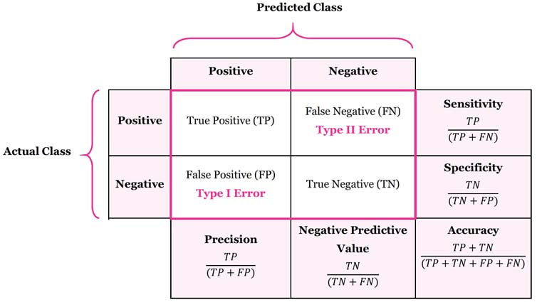
  • Confusion Matrix

    "A confusion matrix is a summary of prediction results on a classification problem. The number of correct and incorrect predictions are summarized with count values and broken down by each class." MachineLearningMastery

    

    source

    • Accuracy

      An error measure of the confusion matrix that is percentage of correct classifications, over the total number of samples.

      $\mathrm{Accuracy} \; =\; \frac{\mathrm{True\; Positives\; +\; True\; Negatives}}{\mathrm{Total}}$

    • Precision - Positive Predictive Value (PPV)

      Considers only one label and counts the percentage of correct classifications on that label.

      • "Precision is undefined for a classifier which makes no positive predictions, that is, classifies everyone as not having diabetes."

      • "When the threshold is very close to 1, precision is also 1, because the classifier is absolutely certain about its predictions."

      • "Precision & recall do not take true negatives into consideration."

      $\mathrm{Precision} \; =\; \frac{\mathrm{True\; Positives}}{\mathrm{True\; Positives} \; +\; \mathrm{False\; Positives}}$
      
        ↳ High Precision = Not many false positives predicted as your positive case

    • Recall - Sensitivity - True Positive Rate (TPR)

      If precision is about the quality of what you got (that is, the quality of the results marked with the label 1), recall is about the quality of what you could have gotten—that is, how many instances of 1  you've been able to extract properly.

      • "A recall of 1 corresponds to a classifier with a low threshold in which all females who contract diabetes were correctly classified as such, at the expense of many misclassifications of those who did not have diabetes."

      $\mathrm{Recall} \; =\; \frac{\mathrm{True\; Positives}}{\mathrm{True\; Positives} \; +\; \mathrm{False\; Negatives}}$
      
        ↳ High Recall = Predicted most of positive case of interest correctly

    • F1 Score

      The harmonic mean of precision & recall.

      $\mathrm{F1\; score} \; =\; 2\left(\frac{\mathit{precision} \; \times \; \mathit{recall}}{\mathit{precision} \; +\; \mathit{recall}}\right)$

    • False Positive Rate (FPR)

      $FPR \; =\; 1 \; -\; \mathrm{Specificity} \; =\; \frac{\mathrm{False\; Positives}}{\mathrm{False\; Positives} \; +\; \mathrm{False\; Negatives}}$

  • ROC (Receiver Operating Characteristics) Curve

    "[The] receiver operating characteristic (ROC) curve is a graph showing the performance of a classification model at all classification thresholds. This curve plots two parameters." Google ML Crash Course

  • AUC (Area Under the ROC Curve)

    "AUC provides an aggregate measure of performance across all possible classification thresholds. One way of interpreting AUC is as the probability that the model ranks a random positive example more highly than a random negative example." Google ML Crash Course

  • Variance Inflation Factor (VIF)

    "[U]sed to detect the presence of multicollinearity . . . VIF measure[s] how much the variance of the estimated regression coefficients are inflated as compared to when the predictor variables are not linearly related." Medium

    $\mathit{VIF} \; =\; \frac{1}{(1 \; -\; R^2)}$

  • Akaike Information criterion (AIC)

    "[A] single number score that can be used to determine which of multiple models is most likely to be the best model for a given dataset. It estimates models relatively, meaning that AIC scores are only useful in comparison with other AIC scores for the same dataset. A lower AIC score is better." AIC is derived from frequentist probability. TowardDataScience

    $\mathit{AIC} \; =\; \mathrm{-2ln}(L) \; +\; 2k$
      ↳ where:
       L = likelihood
       k = # of parameters

  • Bayesian Information Criterion (BIC)

    "[A] criterion for model selection among a finite set of models. It is based, in part, on the likelihood function, & it is closely related to AIC. . . . The BIC resolves this problem by introducing a penalty term for the number of parameters in the model." BIC is derived from Bayesian probability. Analyttica Datalab

    $\mathit{BIC} \; =\; \ln (n)k \; -\; \mathrm{2ln}(\mathit{L̂})$
      ↳ where:
       L̂ = maximized value of likelihood function of the model
       n = # of data points
       k = # of free parameters to be estimated

  • Root Mean Squared Error (RMSE)

    "The standard deviation of the residuals (prediction errors). Residuals are a measure of how far from the regression line data points are; RMSE is a measure of how spread out these residuals are. In other words, it tells you how concentrated the data is around the line of best fit." StatisticsHowTo

    $$\mathrm{RMSE} \; =\; \sqrt{\sum _{n=1}^n\frac{({\mathit{ŷ}}_i \; -\; y_i){\mathrm{}}^2}{n}}$$

• Lasso Regression

  The Lasso algortihm performs regularization by adding to the loss function a penalty term of the absolute value of each coefficient multiplied by some alpha. This is also known as L1 regularization because the regularization term is the L1 norm of the coefficients.
    Similar to Ridge Regression & can be used to select important features of dataset; shrinks the coefficients of less important features to exactly 0.

• Ridge Regression

  Regularized regression where large coefficients are penalized (to avoid over-fitting)

  • Hyperparameter Tuning

    Choosing a set of optimal hyperparameters for a learning algorithm. For example, picking an alpha parameter (α) for Ridge Regression loss function.

  • Regularization

    "In mathematics, statistics, finance, computer science, particularly in machine learning and inverse problems, regularization is the process of adding information in order to solve an ill-posed problem or to prevent overfitting. Regularization can be applied to objective functions in ill-posed optimization problems." Wikipedia

    
    

  • L1 Regularization Norm

    $\mathrm{Loss\; function} \; =\; \mathrm{OLS\; loss\; function} \; +\; \alpha \; *\;$ Σ $\left|a_i\right|$

  • L2 Regularization Norm

    $\mathrm{Loss\; function} \; =\; \mathrm{OLS\; loss\; function} \; +\; \alpha \; *\;$ Σ $a_i{\mathrm{}}^2$

    ↳ where:
    

    ↳ α = constant parameter we choose to penalize for large magnitudes of coefficients (similar to picking k in k-NN) & controls model complexity
    ↳ a = coefficients of linear model
    ↳ OLS = Ordinary Least Squares

  • Elastic Net Regularization

    The penalty is a linear combination of the L1 & L2 penalties.

    $\mathit{Elastic\; Net} \; =\; a \; *\; L1 \; +\; b \; *\; L2$

• Classification & Regression Trees (CART)

  A sequence of if/else questions about individual features with the objective of inferring labels. Trees are capable of capturing non-linear relationships between features & labels. Trees do not require feature scaling such as standardization.

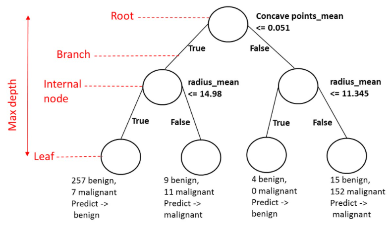
  • Decision Tree

    A data structure consisting of a hierarchy of Nodes (questions or predictions):

    • Nodes

      Grown recursively - based on the known state of its predecessors.

    • Root

      It is the position at which the decision tree starts growing; has no parent node & is a question giving rise to two children nodes.

    • Internal Node

      Has one parent & gives rise to two children.

    • Leaf

      Has one parent node & no children; it is where a prediction is made.

  • Maximum Depth

    Maximum # of branches separating the top from an extreme end.

  • Decision Region

    Region in the feature space where all instances are assigned to one class label.

  • Decision Boundary

    Surface separating different decision regions.

  

  source

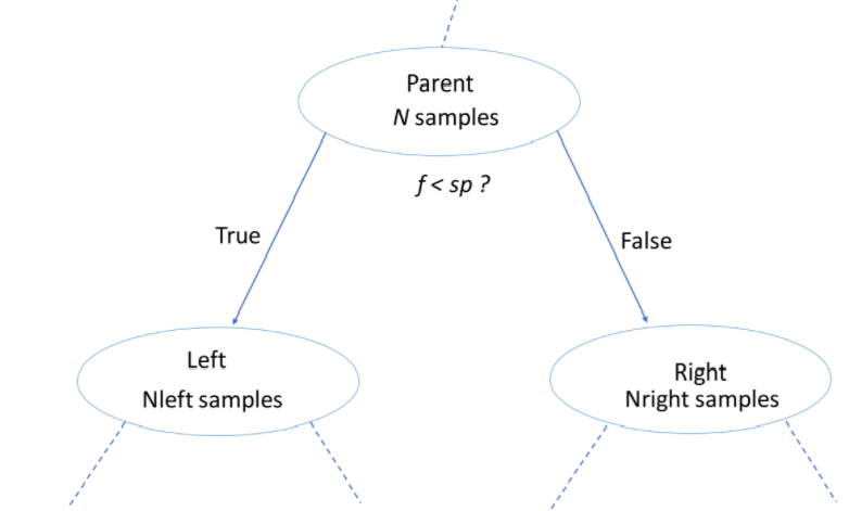
  • Information Gain

    "Information gain is the reduction in entropy or surprise by transforming a dataset and is often used in training decision trees. Information gain is calculated by comparing the entropy of the dataset before and after a transformation" MachineLearningMastery; it is a ratio of information gain to the intrinsic information.

    $\mathit{IG}(f,\; \mathit{sp}) \; =\; I\left(\mathit{parent}\right) \; -\; \left(\frac{N_{\mathit{left}}}{N}I\right(\mathit{left}) \; +\; \frac{N_{\mathit{right}}}{N}I(\mathit{right}\left)\right)$
    ↳ where:
      f = feature
      sp = split point
      impurity criteria = measured via gini index, entropy

  

  source

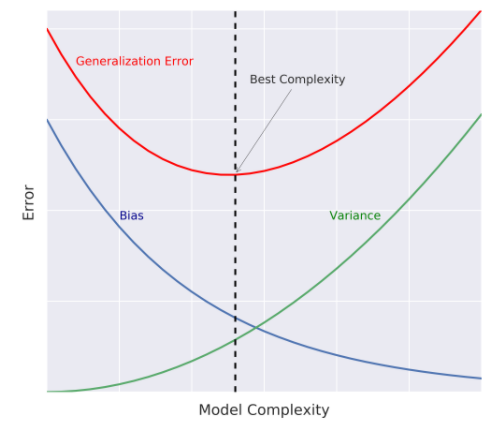
  • Generalization Error

    Does f̂ generelize well to unseen data?

    $\mathit{Generalization\; Error(f̂)} \; =\; {\mathit{bias}}^2 \; +\; \mathit{variance} \; +\; \mathrm{irreducible\; error}$
    ↳ where:
      irreducible error = contribution of noise

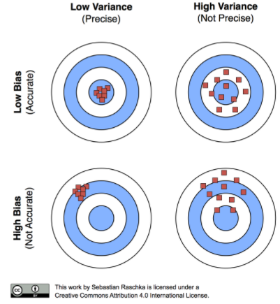
  • Bias

    Bias is an error term that tells you, on average, how much f̂ ≠ f.

    • High-bias models lead to underfitting.

  • Variance

    Variance tells you how much f̂ is inconsistent over different training sets.

    • High-variance models lead to overfitting.

  • Model Complexity

    Sets the flexibility to approximate the true function of f̂.

  

  source

  

  source

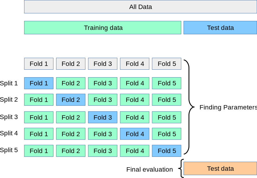
  • Cross-Validation

    "a resampling procedure used to evaluate machine learning models on a limited data sample. ... That is, to use a limited sample in order to estimate how the model is expected to perform in general when used to make predictions on data not used during the training of the model." MachineLearningMastery
    To combat limited ability with current dataset to generalize to unseen data.

    • K-Fold CV Error

      $\mathrm{CV\; error} \; =\; \frac{E_1 \; +\; .\; .\; . \; +\; E_{10}}{10}$

  

  source

  • Decision Tree Regression

    Supervised learning algorithm used for classification problems; works for categorical & continuous variables

    • Standard Deviation Reduction

    F(T, X) = ΣP(c)S(c)

  • Limitations of CARTs

    • Classification: can only produce orthogonal decision boundaries.

    • Sensitive to small variations in the training set.

    • High variance: unconstrained CARTs may overfit the training set.

• Ensemble Learning

  Ensemble methods use multiple learning algorithms to obtain better predictive performance than could be obtained from any of the constituent learning algorithms alone.

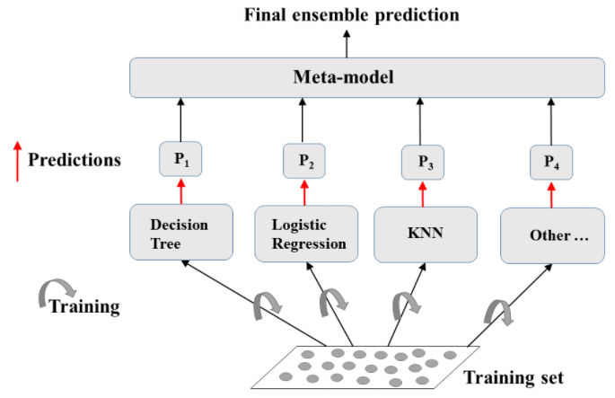
  • Voting Classifier

    • Train different models on the same datset.

    • Let each model make its predictions.

    • Meta model: aggregates predictions of individual models.

    • Final prediction: more robust & less prone to errors.

    • Best results: models are skillful in different ways.

  

  source

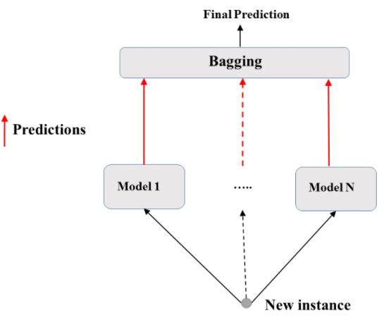
  • Bagging: Bootstrap Aggregating

    • Train different subests of the same training set with same algorithm in N models.

    • Base estimator: Decision Tree, Logistic Regression, Neural Net . . .

    • Each estimator is trained on a distinct bootstrap sample of the training set.

    • Estimators use all available features for training & prediction.

    • Reduces variance of individual models in the ensemble.

  

  source

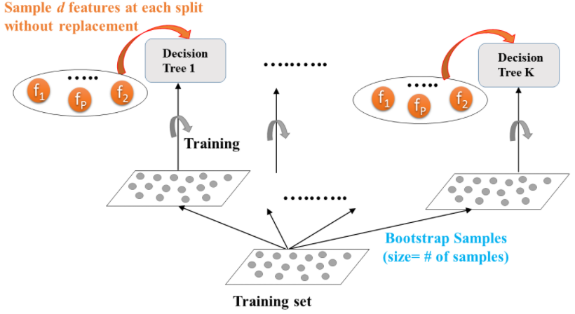
  • Random Forests

    • Base estimator: Decision Tree

    • Each estimator is trained on a different bootstrap sample having the same size as the training set.

    • Introduces further randomization in the training of individual trees.

    • d features are sampled at each node without replacement.
      ↳ where: d < total # of features

  

  source

  • Boosting

    Ensemble method combing several weak learners to form a strong learner.
    ↳ where: weak learner = slightly better than random guessing ⇒ the proverbial dart-throwing monkey.

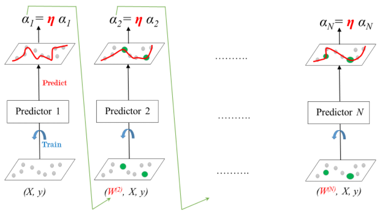
    • AdaBoost: Adaptive Boosting

      • Each predictor pays more attention to the instances wrongly predicted by its predecessors.

      • Achieved by constantly changing the weights of training instances.

      • Each predictor is assigned a coefficient α.

      • α depends on the predictor's training error.

      • Leanring Rate: 0 < η ≤ 1

    

    source

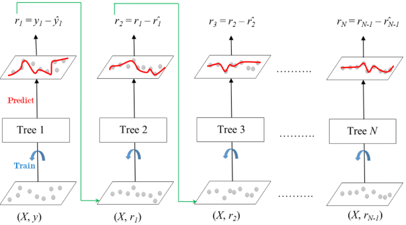
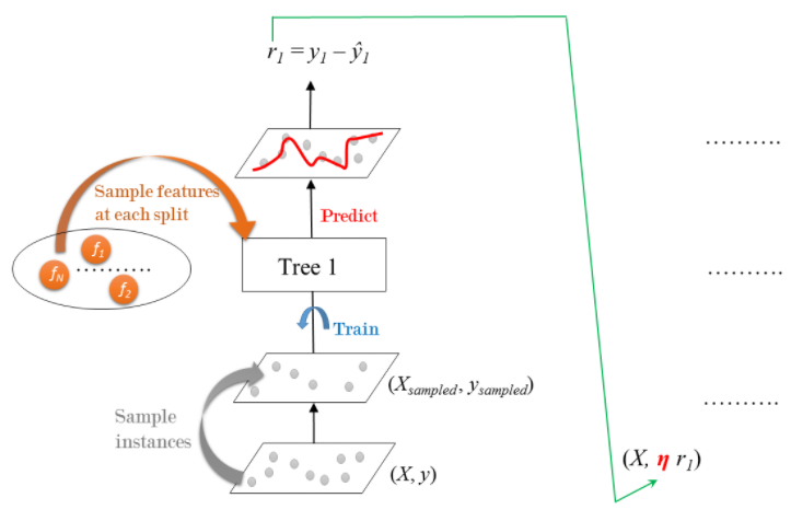
    • Gradient Boosting

      • Sequential correction of predecessor's errors.

      • Does not tweak the weights of training instances.

      • Fit: each predictor is trained using its predecessor's residual errors as labels.

      • Gradient Boosted Trees: a CART is used as base learner.

    

    source

    • Stochastic Gradient Boosting

      • Each tree is trained on a random subset of rows of the training data.

      • The samples instances (40%-80% of the training set) are sampled without replacement.

      • Features are sampled (without replacement) when choosing split points.

      • Result: further ensemble diversity.

      • Effect: adding further variance to the ensemble of trees.

    

    source

  • Hyperparameters

    Parameters are learned from data & include CART examples such as split-point of node & split-feature of node. Hyperparameters are not learned from the data & must be set prior to training. CART examples include maximum depth, minimum samples leaf & splitting criterion.
    Approaches include:

    • Grid Search

      • Manually set a grid of discrete Hyperparameter values.

      • Set a metric for scoring model performance.

      • Search exhaustively through the grid.

      • For each set of hyperparameters, evaluate each model's CV score.

      • The optimal hyperparameters are those of the model achieving the best CV score.

      • Suffers from the curse of dimensionality ⇒ the bigger the grid the longer it takes to find the solution.

    • Random Search

    • Bayesian Optimization

    • Genetic Algorithms

• Support Vector Machines

  Discriminative classifier formally defined by a separating hyperplane

  • Maximum Margin Hyperplane | Support Vectors

  {x_i, y_i} where i = 1 . . . L, y_i ∈ {-1, 1}, x ∈ ℝ^D

• Kernel SVM

Mapping to a higher-dimensional space, applying the support vector algorithm & then projecting back to lower dimensional space resulting in a nonlinear separator

• Linearly Separable with Hyperplane in 3D

φ(x₁, x₂) ⇒ (x₁, x₂, z)

• The Gaussian or Radial Basis Function (RBF) Kernel

$K(\mathrm{x⃗,\; }{\mathrm{l⃗}}^{\mathrm{ i}})=\exp (-\frac{\mathrm{||\; x⃗,\; }{\mathrm{l⃗}}^{\mathrm{ i}}{\mathrm{||}}^2}{2{\sigma }^2})$


↳ where:


↳ K = function applied to two vectors
↳ x = point in datasets
↳ l = landmark

• Sigmoid Kernel

K(X, Y) = tanh(γ ˙ X^TY + r)

• Polynomial Kernel

K(X, Y) = tanh(γ ˙ X^TY + r)^d, γ > 0

• Naive Bayes Classification

  Probabilistic classifier based on Bayes Theorem with an assumption of independence between predictors (aka, features or independent variables)

  • Bayes Theorem ⇒ The probability of an event given prior knowledge of related events that occurred earlier

    $P(y\mid x_1,\dots ,x_n)=\frac{P(y)P(x_1,\dots ,x_n\mid y)}{P(x_1,\dots ,x_n)}$

• K-Nearest Neighbors

  An algorithm that predicts the label of a data point in both classification & regression.   The algorithm stores all available cases & classifies new cases by a "majority vote" of its K-nearest neighbors

  • Euclidean Distance

    $\mathrm{Between}{P}_1\&P_2=\sqrt{(x_2-x_1)2^{}+(y_2-y_1)2^{}}$

Unsupervised Learning

"Looks for previously undetected patterns in a data set with no pre-existing labels and with a minimum of human supervision"
"[P]resent examples without any hint, leaving it to the algorithm to create a label. For instance, when we need to figure out how the groups inside a customer database can be partitioned into similar segments based on their characteristics and behaviors." WGU MSDA

• K-Means Clustering

Unsupervised algorithm which solves clustering problems; follows simple/easy way to classify a dataset through a certain number of clusters

• Within Cluster Sum of Squares (WCSS)| Quantifiable metric to evaluate how certain number of clusters performs compared to different number of clusters

WCSS = Σ distance(P_i, C₁)² + Σ distance(P_i, C₂)² +Σ distance(P_i, C₃)²

↳ where:


↳ distance = distance between each point inside cluster
↳ C = centroids, respectively


• Apriori Association

Analyzes the association of specific preferences in customer transactions (movies watched, items purchased in convenience store - beer & pampers urban myth) to discover relationships and how items are associated with each other

• Support

Movie recommendation example:
  ↳ where M = specific Movie

$\mathrm{Support(M)}=\frac{\mathrm{\#\; of\; user\; watchlists\; containing\; M}}{\mathrm{\#\; of\; user\; watchlists}}$

• Confidence

$\mathrm{Confidence}(M_1\to M_2)=\frac{\mathrm{\#\; of\; user\; watchlists\; containing}(M_1\to M_2)}{\mathrm{\#\; of\; user\; watchlists\; containing}(M_1)}$


• Lift → measuring the relevance of an associated rule & the improvement prediction

$\mathrm{Lift}(M_1\to M_2)=\frac{\mathrm{Confidence}(M_1\to M_2)}{\mathrm{Support}(M_2)}$

Reinforcement Learning

"how software agents ought to take actions in an environment in order to maximize the notion of cumulative reward"
"[P]resent examples without labels, as in unsupervised learning, but get feedback from the environment as to whether label guessing is correct or not. For instance, when we need software to act successfully in a competitive setting, such as a videogame or the stock market, we can use reinforcement learning. In this case, the software will then start acting in the setting and it will learn directly from its errors until it finds a set of rules that ensure its success." WGU MSDA

• Upper Confidence Bound Algorithm | Deterministic Model

Modern application of Multi-Armed Bandit Problem (reference slot machine distributions)

• Advertising Model (requires update at every round)

Step 1: Each round n considers two numbers for each ad i:


  ↳ N_i(n) → # of times the ad i selected up to round n
  ↳ R_i(n) → Σ of rewards of ad i up to round n



Step 2: From these two numbers we compute:


  ↳ Average reward of ad i up to round n with:

        $\mathrm{r̄}(n)=\frac{R_{\mathrm{i}}(n)}{N_{\mathrm{i}}(n)}$


  ↳ Confidence interval [r̄_i(n) - △_i(n), r̄_i(n) + △_i(n)] at round n with:

        ${△}_{\mathrm{i}}(n)=\sqrt{\frac{3}{2}*\frac{\log (n)}{N_{\mathrm{i}}(n)}}$


Step 3: Select the ad i that has the maximum UCB r̄_i(n) + △_i(n)

• Thompson Sampling Algorithm | Probabilistic Model

Constructs distributions of where we think the actual expected value might lie; an auxiliary mechanism to solve the problem

• Advertising Model (can accomodate delayed feedback & has better empirical evidence than UCB)

Step 1: Each round n considers two numbers for each ad i:


  ↳ N_i¹(n) → # of times the ad i rewarded 1 up to round n
  ↳ N_i⁰(n) → # of times the ad i rewarded 0 up to round n



Step 2: For each ad i, we take a random draw from the distribution below:



θ_i(n) = β(N_i¹(n) + 1, N_i⁰(n + 1))




Step 3: Select the ad i that has highest θ_i(n)

• Random Forest Regression

Ensemble decision trees; a collection of decision trees (aka forest) to classify a new object based on attributes; each tree gives a classification & we say the tree "votes" for the class

• Dimensionality Reduction

Identifies highly significant variables when you have thousands

• Gradient Boosting

Ensemble of machine learning algorithms

Lovely Deep Learning

"[M]achine learning uses multiple layers of simple, adjustable computing elements." (Russell, p. 26)
"Deep learning solves [the] central problem in representation learning by introducing . . . simpler representations . . . [and] enables the computer to build complex concepts out of simpler concepts . . . breaking the desired complicated mapping into a series of nested simple mappings . . . called "hidden [layers]" because their values are not given in the data." (Bengio, p. 5-6)

Mathematics

Etymology: The word "mathematics" comes from Ancient Greek máthēma (μάθημα), meaning "that which is learnt," "what one gets to know," hence also "study" and "science". Wikipedia

Intimate Linear Algebra

The study of linear equations & geometric transformations using matrices, vectors spaces & determinants.
"Solving for unknowns within a system of linear equations." Mathematical Foundations of Machine Learning

Fundamental Mathematical Objects

• Scalars

  A scalar is simply a single number, in contrast to the other mathematical objects studied in linear algebra. A scalar can be thought of a matrix with a single entry. (Goodfellow, pg. 29)

• Vectors

  A vector is an array of numbers. Vectors can be thought of matrices that contain only one column. (Goodfellow, pg. 30)

• Matrix

  A matrix is an a two dimensional array of numbers such that each element is identified by two indices instead of just one. (Goodfellow, pg. 30)

  • Transpose

    "[T]he mirror image of a matrix across a diagonal line. The transpose of a vector is therefore a matrix with only one row" (Goodfellow, pg. 31).

  • Matrix product

    Perhaps the most important operation of matrices is their multiplication. The matrix product of matrices A and B is a third matrix C.

    $C \; =\; AB\hspace{0.5em}\; \Rightarrow \; \hspace{0.5em}{C}_i{}_{,}{}_j \; =\;$ Σ $A_i{}_{,}{}_k{B}_k{}_{,}{}_j$

• Tensor

  "In some cases we will need an array with more than two axes. . . . [A]n array of numbers arranged on a regular grid with a variable number of axes . . ." (Goodfellow, pg. 31)
    In an n-dimensional space a tensor of rank n is a mathematical object that has n indices, mⁿ components and obeys certain transformation rules.

• Matrix Notation

  $\mathrm{Y} \; =\; \mathrm{X}\mathrm{\beta } \; +\; \mathrm{\epsilon }$

• Sparse Matrix

  In numerical analysis and scientific computing, a sparse matrix or sparse array is a matrix in which most of the elements are zero.

Linear Regression

• Matrix-Vector Multiplication Function

  $\left[\begin{array}{c}{y}_1\\ y_2\end{array}\right] \; =\; \left[\begin{array}{cccc}1& x_{11}& x_{12}& x_{13}\\ 1& x_{21}& x_{22}& x_{23}\end{array}\right]\left[\begin{array}{c}{\beta }_0\\ {\beta }_1\\ {\beta }_2\\ {\beta }_3\end{array}\right] \; +\; \left[\begin{array}{c}{\epsilon }_1\\ {\epsilon }_2\end{array}\right]$
    ↳ where:
        $\mathrm{Vector\; of\; Outcomes\; for\; Each\; Case} \; =\; \left[\begin{array}{c}{y}_1\\ y_2\end{array}\right]$
        $\mathrm{Matrix\; of\; Scores\; for\; Each\; Case} \; =\; \left[\begin{array}{cccc}1& x_{11}& x_{12}& x_{13}\\ 1& x_{21}& x_{22}& x_{23}\end{array}\right]$
        $\mathrm{Vector\; of\; Regression\; Coefficients\; (y-intercept\; \&\; slopes)} \; =\; \left[\begin{array}{c}{\beta }_0\\ {\beta }_1\\ {\beta }_2\\ {\beta }_3\end{array}\right]$
        $\mathrm{Vector\; of\; Error\; Terms} \; =\; \left[\begin{array}{c}{\epsilon }_1\\ {\epsilon }_2\end{array}\right]$

Determinants

  ↳ The volume scaling factor of the linear transformation described by the matrix

• Square Matrices

  • Determinant Equation 2x2 Matrix

    $\left|\begin{array}{cc}\mathrm{a}& \mathrm{b}\\ \mathrm{c}& \mathrm{d}\end{array}\right| \; =\; \mathrm{ad} \; -\; \mathrm{bc}$

  • Trace of Matrix

    Equal to the sum of the values along the main diagonal

    $\mathrm{Trace}\left[\begin{array}{cc}\mathrm{a}& \mathrm{b}\\ \mathrm{c}& \mathrm{d}\end{array}\right] \; =\; \mathrm{a} \; +\; \mathrm{d}$

Geometrical Aspects of Linear Algebra

  ↳ Mathematics to used see through to the governing dynamics of the physical universe

• Orthogonality & Change of Basis

  • Least Squares Solution

    $A^{\mathrm{T}}A{\mathrm{x⃗}}^{\mathrm{*}}=A^{\mathrm{T}}\mathrm{b⃗}$

• Orthonormal Bases

  • Orthogonality

    Every vector in set is orthogonal to every other vector in set; as perpendicular is to two-dimensional space (vectors at 90° angle), orthogonal is to three- or n-dimensional space.

    ${\mathrm{v⃗}}_1\cdot {\mathrm{v⃗}}_2 \; =\; 0$

  • Normality

    Every vector has been normalized; every vector has a length of 1.

    ${\mathrm{v⃗}}_1\cdot {\mathrm{v⃗}}_1 \; =\; \parallel {\mathrm{v⃗}}_1\parallel {}^2 \; =\; 1$

  • Projection onto an Orthonormal Basis

    Using an orthonormal subspace drastically simplifies projection equation from:

    ${\mathrm{Proj}}_{\mathrm{v}}\mathrm{x⃗} \; =\; A\left({\mathrm{A}}^{\mathrm{T}}\mathrm{A}\right){\mathrm{}}^{-1}{\mathrm{A}}^{\mathrm{T}}\mathrm{x⃗}$
         ↓
    ${\mathrm{Proj}}_{\mathrm{v}}\mathrm{x⃗} \; =\; \mathrm{A}{\mathrm{A}}^{\mathrm{T}}\mathrm{x⃗}$

  • Gram-Schmidt Process

    Converts non-orthonormal set into an orthonormal set

    $\mathrm{Subspace\; v} \; =\; \mathrm{span}\left({\mathrm{v⃗}}_1\mathrm{,\; }{\mathrm{v⃗}}_2\mathrm{,\; }{\mathrm{v⃗}}_3\right)\mathrm{\hspace{1em}\hspace{1em}\hspace{1em}\hspace{1em}Step\; 1:\; \hspace{1em}}{\mathrm{u⃗}}_1 \; =\; \frac{{\mathrm{v⃗}}_1}{\mathrm{\parallel }{\mathrm{v⃗}}_1\mathrm{\parallel }}$
          $\; =\; \mathrm{span}\left({\mathrm{u⃗}}_1\mathrm{,\; }{\mathrm{v⃗}}_2\mathrm{,\; }{\mathrm{v⃗}}_3\right)\mathrm{\hspace{1em}\hspace{1em}\hspace{1em}\hspace{1em}\; Step\; 2:\; \hspace{1em}}{\mathrm{w⃗}}_2 \; =\; {\mathrm{v⃗}}_2 \; -\; ({\mathrm{v⃗}}_2 \; \cdot \; {\mathrm{u⃗}}_1){\mathrm{u⃗}}_1$
          $\; =\; \mathrm{span}\left({\mathrm{u⃗}}_1\mathrm{,\; }{\mathrm{u⃗}}_2\mathrm{,\; }{\mathrm{v⃗}}_3\right)\mathrm{\hspace{1em}\hspace{1em}\hspace{1em}\hspace{1em}\; Step\; 3:\; \hspace{1em}}{\mathrm{w⃗}}_3 \; =\; {\mathrm{v⃗}}_3 \; -\; \left[\right({\mathrm{v⃗}}_3 \; \cdot \; {\mathrm{u⃗}}_1){\mathrm{u⃗}}_1 \; +\; ({\mathrm{v⃗}}_3 \; \cdot \; {\mathrm{u⃗}}_2\left){\mathrm{u⃗}}_2\right]$
          $\; =\; \mathrm{span}\left({\mathrm{u⃗}}_1\mathrm{,\; }{\mathrm{u⃗}}_2\mathrm{,\; }{\mathrm{u⃗}}_3\right)$

• Eigenvalues & Eigenvectors

  Literally "special" or "self" values/vectors that correspond to a matrix or linear transformation; a way to diagonalize a problem, adjusting specific parts without disturbing others

  • Eigenvector Transformation ( Brilliant 3Blue1Brown visualization)

    $\mathrm{T(v⃗)} \; =\; \mathrm{Av⃗}$
    $\mathrm{T(v⃗)} \; =\; \mathrm{\lambda v⃗}$
      ↳ where:
          $\lambda \; =\; \mathrm{eigenvalue;\; a\; scalar}$
          $\mathrm{v⃗} \; =\; \mathrm{eigenvector}$
    $\therefore \; \mathrm{Av⃗} \; =\; \mathrm{\lambda v⃗}$
      ↳ algebraically:
          $0⃗ \; =\; (\lambda {\mathrm{I}}_{\mathrm{n}} \; -\; A)\mathrm{v⃗}$

  • Eigenspace (E_λ)

    ${\mathrm{E}}_{\mathrm{\lambda }} \; =\; \mathrm{N}(\mathrm{\lambda }{\mathrm{I}}_{\mathrm{n}} \; -\; \mathrm{A})$
      ↳ where:
      $\mathrm{N} \; =\; \mathrm{Null\; Space}$
      ${\mathrm{I}}_{\mathrm{n}} \; =\; \mathrm{Identity\; Matrix}$

• Fast Fourier Transformation

  "A fast Fourier transform is an algorithm that computes the discrete Fourier transform of a sequence, or its inverse. Fourier analysis converts a signal from its original domain to a representation in the frequency domain and vice versa." Wikipedia

Salient Statistics & Probabilities

Statistics is the art of making numerical conjectures about puzzling questions.
↳ Is statistics a field of mathematics? Some say it is not mathematics but the science of data. Whatever you decide, you must embrace it, my Dear Friends.

Terminology

• Index: a descriptive statistic made up of other descriptive statistics that consolidates lots of information into a single number

Probability

Generalizing logic to situations with uncertain outcomes & measurements, & incomplete theories; the possible outcomes of events.
"The formalization of probability, combined with the availability of data, led to the emergence of statistics as a field." Artificial Intelligence: A Modern Approach, pg 8

• Basic Formulae

• Probability of an Event

$\mathrm{P(A)}=\frac{\mathrm{Outcome(s)\; You\; Are\; Looking\; For}}{\mathrm{Total\; Possible\; Outcomes}}\Rightarrow \frac{\mathrm{Event}}{\mathrm{Sample\; space}}\Rightarrow \frac{\mathrm{A,\; B,\; etc.}}{S}$

• Complement of an Event

$\mathrm{P(Ā)}=\mathrm{1\; -\; P(A)}$

• Union(∪, Or) & Intersection(∩, And)

P(A ∪ B) = P(A) + P(B) - P(A ∩ B)

• Permutations & Combinations

  • The Combinatorial Explosion

    $P(n,r) \; =\; \frac{n!}{(n \; -\; r)!}$

• Bayes' Theorem

  Tells the probability of an event given prior knowledge of related events that occurred earlier

  • Bayesian Analysis: Probability of B given A

    $\mathrm{Posterior} \; =\; \frac{\mathrm{likelihood\; *\; prior}}{\mathrm{marginal}}$
    
    $\mathrm{P}\left(\mathrm{A\; |\; B}\right) \; =\; \frac{\mathrm{P}\left(\mathrm{B\; |\; A}\right) \; *\; \mathrm{P}\left(\mathrm{A}\right)}{\mathrm{P}\left(\mathrm{B}\right)}$
      ↳ where:
      A       = cause event
      B       = effect event
      P(A|B)   = probability of cause A given effect B is true
      P(B|A)   = probability of effect B given cause A is true
      P(A), P(B) = independent probabilities of effect A & cause B

• Random Walk

  "A process for determining the probable location of a point subject to random motions, given the probabilities (the same at each step) of moving some distance in some direction. Random walks are an example of Markov processes, in which future behaviour is independent of past history."

• Drunkard's Walk

  "A typical example is the drunkard’s walk, in which a point beginning at the origin of the Euclidean plane moves a distance of one unit for each unit of time, the direction of motion, however, being random at each step. The problem is to find, after some fixed time, the probability distribution function of the distance of the point from the origin. Many economists believe that stock market fluctuations, at least over the short run, are random walks." This is observed in Brownian Motion.

Dynamic Calculus

The mathematics of curves, motion and change, calculus is basically very advanced algebra (finding rates & slopes) & geometry (addition to infinity & finding area).

Three Central Problems of Calculus

• Forward Problem: given a curve, find its slope everywhere

• Backward Problem: given the slope everywhere, find the curve

• Area Problem: given the curve, find the area under it

Fundamental Theorem of Calculus (FTC)

Shows the relationship between differentiation & integration. If a function is integrated & then differentiated, it is back to the original function. Integration & differentiation are inverse to each other.

• Part 1

  • Differentiation

    $\mathrm{If\; }r\left(x\right)\mathrm{is\; continuous\; on\; }[a, b] \mathrm{then}$
    
      $f\left(x\right) \; =\; {\int }^{\mathrm{b}}r\left(t\right) dt$
    
    $\mathrm{is\; continuous\; on\; }[a, b], \mathrm{it\; is\; differentiable\; on\; }(a, b), \mathrm{and}$
    
      $f\prime \left(x\right) \; =\; r\left(x\right)$

Differentiation

The derivative function tells how fast & where the function is increasing or decreasing.

• Derivatives

  Finding the slope of a function at a specific point.

  • f′(x) or $\frac{dy}{dx}$

    $\mathrm{f\prime (x)} \; =\;$lim $\frac{\mathrm{f(x\; +\; h)\; -f(x)}}{\mathrm{h}}$
      ↳ where:
      $\mathrm{h} \; =\; {\mathrm{x}}_2 \; -\; {\mathrm{x}}_1$

Integration

The integral of a function models the area under the graph of a function.

• Antiderivatives & Indefinite Integrals

  Find the area under the curve everywhere, over the entire domain of the function; the interval is unbounded & there are no limits on the interval.

  • Integral for Basic Power Functions

    $\int {\mathrm{x}}^{\mathrm{a}}dx \; =\; \frac{{\mathrm{x}}^{\mathrm{a\; +\; 1}}}{\mathrm{a\; +\; 1}}$

• Definite Integrals

  • The Interval

    Find the area under the curve over a specific interval, at the limits of integration.

    ${\int }^{\mathrm{b}}f\mathrm{(x)} dx \; =\; \mathrm{F(b)\; -\; F(a)}$

• Riemann Sums

  Way to geometrically estimate the area under a curve: divide the area into many thin rectangles, find the subsequent areas & then sum those areas

  • Summation Notation

    $$Σ ( n - 1 ) ( n + 2 )   =   ${\mathrm{a}}_{\mathrm{n}}$

  • Expanding Series

    $$Σ $\frac{1}{n^2} \; =\;$ ${\mathrm{a}}_{\mathrm{n}}$
    $\hspace{1em}\hspace{1em}\hspace{1em}\; =\; \frac{1}{1^2} \; +\; \frac{1}{2^2} \; +\; \frac{1}{3^2} \; +\; \frac{1}{4^2} \; +\; \frac{1}{5^2} \; +\; \frac{1}{6^2}$
    $\hspace{1em}\hspace{1em}\hspace{1em}\; =\; 1 \; +\; \frac{1}{4} \; +\; \frac{1}{9} \; +\; \frac{1}{16} \; +\; \frac{1}{25} \; +\; \frac{1}{36}$

  • Riemann Sum Formula

    Use midpoints, left or right endpoints of finite # of rectangles to estimate the area under the curve

    $R_n \; =\;$Σ $f\left(x_i\right)\mathrm{\Delta }x$
    
      ↳ expanded:
    
    $R_n \; =\; \mathrm{\Delta }x\left[f\right(x_1) \; +\; f(x_2) \; +.\; .\; .+\; f(x_n\left)\right]$
    
      ↳ where:
      $\mathrm{\Delta }x \; =\; \frac{b \; -\; a}{n} \; =\; \mathrm{width\; of\; subinterval/rectangle}$
      $f\left(x_i\right) \; =\; \mathrm{length\; of\; rectangle}$
      $n \; =\; \mathrm{\#\; of\; subintervals}$

  • Midpoint Rule

    $M_n \; =\; \frac{b \; -\; a}{n}\left[f\right(\frac{x_0 \; +\; x_1}{2}) \; +\; f(\frac{x_1 \; +\; x_2}{2}) \; +\; f(\frac{x_2 \; +\; x_3}{2}).\; .\; . \; +\; f(\frac{x_{\mathrm{n\; -\; 1}} \; +\; x_n}{2}\left)\right]$

• Other Approximation Methods

  • Limit Process to Find Area

    ${\int }^{\mathrm{b}}f\mathrm{(x)} dx \; =\;$ $$lim Σ $f\left(x_i\right)\mathrm{\Delta }x$
    
    Step 1:  define width of subinterval or Δx
       ↳ $\Delta x \; =\; \frac{b \; -\; a}{n}$
    
    Step 2:  define x_i as # of subintervals
       ↳ $x_i \; =\; a \; +\; i\Delta x$
    
    Step 3:  apply summation notation for i, i² & i³ as series
       ↳ $$Σ $i \; =\; \frac{\mathrm{n(n\; +\; 1)}}{2}$
       ↳ $$Σ $i^2$ $\; =\; \frac{\mathrm{n(n\; +\; 1)(2n\; +\; 1)}}{6}$
       ↳ $$Σ $i^3$ $\; =\; \frac{n^2\mathrm{(n\; +\; 1)}{\mathrm{}}^2}{4}$

  • Trapezoidal Rule

    Approximating area under curve may be more accurate because trapezoids get closer to the actual curve than rectangles

    ${\int }^{\mathrm{b}}f\mathrm{(x)} dx \; \approx \; \frac{\mathrm{\Delta }x}{2}\left[f\right(x_0) \; +\; 2f(x_1) \; +\; 2f(x_2) \; +\; .\; .\; . \; +\; 2f(x_{\mathrm{n-2}}) \; +\; 2f(x_{\mathrm{n-1}}) \; +\; f(x_n\left)\right]$

  • Simpson's Rule

    The value of n must be even

    $S_n \; =\; \frac{\mathrm{\Delta }x}{3}\left[f\right(y_0) \; +\; 4f(y_1) \; +\; 2f(y_2) \; +\; 4f(y_3) \; +\; .\; .\; . \; +\; 2f(y_{\mathrm{n-2}}) \; +\; 4f(y_{\mathrm{n-1}}) \; +\; f(y_n\left)\right]$

• Error Bounds

  Largest possible value of error of approximation; level of reliability

  • Midpoint Rule (E_M)

    $\left|E_M\right| \; \le \; \frac{K(\mathrm{b\; }-\mathrm{ \; a}){\mathrm{}}^3}{24n^2}\hspace{1em}\; |f^{″}\left(x\right)| \; \le \; K$

  • Trapezoidal Rule (E_T)

    $\left|E_T\right| \; \le \; \frac{K(\mathrm{b\; }-\mathrm{ \; a}){\mathrm{}}^3}{12n^2}\hspace{1em}\; |f^{″}\left(x\right)| \; \le \; K$

• Integration by Parts Formula

  Using u substitution to simplify our integral to make it easier to evalutate.

  $\int \mathit{udv} \; =\; \mathit{uv} \; -\; \int \mathit{vdu}$

Computer Science Mathematics

Absolute Value Inequalities

• Absolute Value of a Function

  • Less Than a

    Closer to zero than a

    $\left|f\right(x\left)\right| \; <\; a$
    $f\left(x\right)>-a\mathrm{\hspace{0.5em}\; and\; \hspace{0.5em}}f\left(x\right)<a$
    $-a<f\left(x\right)<a$
    $(-a,a)$

  • Greater Than a

    Further away from zero than a

    $\left|f\right(x\left)\right| \; >\; a$
    $f\left(x\right)>a\mathrm{\hspace{0.5em}\; or\; \hspace{0.5em}}f\left(x\right)<-a$

Scientific Notation

Any number can be written in scientific notation. It involves shifting the decimal place to the left (positive) or right (negative) until the result is a number with only one place before the decimal point & then multiplying by 10 raised to the number of places shifted.

• Notation Process Result

  1. A decimal number less than 10 and greater than 1 multiplied by,

  2. 10 raised to a specific whole number

• Example:

  $\mathrm{\hspace{1em}\hspace{0.5em}1.17E} \; +\; 07 \; =\; 1.17 \; *\; {10}^7 \; =\; \mathrm{11,700,000}$

NP Complete Problem

"We call these problems "nondeterministic polynomial" or NP, because you can't give someone a pre-determined set of steps to solve it (unless that someone is a perfect guesser!), but if someone does happen to solve it, they would only need a polynomial number of steps. . . .
  [W]e can find the answer to any NP problem by solving a related problem in this group. The problems in this group are called "NP-complete" (because solving one of them can solve the complete group of NP problems). If we ever found a fast (i.e. polynomial) way to solve any NP-complete problem, we could find fast ways to solve every NP problem. Then we wouldn't have to talk about NP any more, because they would all just be P (polynomial) problems. That's why we call the problem "P=NP". . . .
  [M]athematicians think that NP-complete problems are not P, because so many people have spent so much time thinking about it that if they were, somebody would have found out how by now (because it's usually easier to find a way to do something than to prove that there is no way)." Reddit ELI5

• P: The set of all problems that can be solved in polynomial time (polynomial in relation to the input) by a deterministic Turing machine.

• NP: The set of all problems that can be solved in polynomial time if you have a non-deterministic Turing machine. That is, if you have a magical computer that can perform both actions at a decision point simultaneously. However, given a proposed solution to a problem in NP, that solution can be verified in polynomial time by a normal, deterministic Turing machine.

• NP-hard: The set of all problems that any problem in NP can be reduced to in polynomial time.

• NP-complete: The set of problems that any problem in NP can be reduced to in polynomial time, whose solutions can still be verified in polynomial time. This is the subset of NP-hard that overlaps NP. Generally-speaking, the set of NP-complete problems is a kind of "upper bound" on the complexity of NP problems. Every NP problem can be solved by an NP-complete problem, and the solution can be verified in polynomial time.

Marvelous Logarithms

Logarithms were the supercomputers their era.   See the Description of the Marvelous Canon of Logarithms by John Napier

• Rule of Logs: the log of a product is the sum of the logs
  Logarithms undo the actions of exponential functions. Logarithms & exponentials are inverse functions

• Inverse of an Exponential Function

  y = a^x   ⇒   x = a^y
  100 = 10²   ⇒   log₁₀ of 100 = 2

• Logarithmic Function

  ""[S]imply an exponential function with the x & y axes swtitched. In other words, the up-and-down direction on an exponential graph corresponds to the right-and-left direction on a logarithmic graph, & the right-and-left direction on an exponential graph corresponds to the up-and-down direction on a logarithmic graph." (Ryan, p. 59)

• The relationship of exponetial to logarithmic

  (the exponential function) x = a^y   ⇒   log_a of x = y (the logarithmic function)

• The Binary Logarithm

  Log² n is the power to which the number 2 must be raised to obtain the value n.
  For any real number x:

  $x \; =\; {\log }_2\mathrm{ n}\hspace{1em}\; \iff \; \hspace{1em}{2}^x \; =\; n$

Cordially Discrete Mathematics

Branch of mathematics dealing with discrete (distinct & disconnected) or finite sets of elements rather than continuous or infinite sets of elements. The terms discrete & continuous are analogous to the computer science terms digital & analog.
* Brilliant course from Shawn Grooms at freeCodeCamp: Math for Programmers

• Set of Natural Numbers

  ℕ = {1, 2, 3, . . .}   ⇒   The set of Natural Numbers (Cardinal or Counting Numbers) include all positive, non-zero integers.

• Set of Integers

  ℤ = {. . . , -1, 0, 1, . . .}

• Set of Rational Numbers

  $\mathbb{Q}\mathrm{ \; =\; }\{\frac{a}{b} \; :\; a,\; b \; \in \; \; \mathbb{Z},\; b \; \ne \; 0\}$  ⇒   The set of Rational Numbers include ratios of two integers where the denominator is non-zero.

• Binary Operators for Sets

  • For Sets:

    A = {x, y, z}
    B = {c, x, y}

  • Union

    $\mathrm{A} \; \cup \; \mathrm{B}=\{p:\; p \; \in \; \mathrm{A}\mathrm{ \; or\; }p \; \in \; \mathrm{B}\}$  ⇒   A union B equals the set containing elements p, such that p is an element of A or p is an element of B.

  • Intersection

    $\mathrm{A} \; \cap \; \mathrm{B}=\{p:\; p \; \in \; \mathrm{A}\mathrm{ \; and\; }p \; \in \; \mathrm{B}\}$  ⇒   A intersection B equals the set containing elements p, such that p is an element of A and p is an element of B.

• Logic

  Logic is a systematic way of thinking that allows us to deduce new information from old information & to parse the meaning of sentences.

  Logic   ⇒   Mathematics   ⇒   Algorithms   ⇒   Code

• The Universal Set

  The Universe is the maximum boundary of extant sets; it is the largest set; everything outside the Universal Set does not exist.
  If the Universel Set is not defined, we assume it to be the set of Real Numbers (ℝ).

• Associativity

  We can regroup the sets we are talking about - it does not matter where we put our parentheses.

  $\mathrm{A} \; \cup \; (\mathrm{B} \; \cup \; \mathrm{C}) \; =\; (\mathrm{A} \; \cup \; \mathrm{B}) \; \cup \; \mathrm{C}$
  $\mathrm{A} \; \cap \; (\mathrm{B} \; \cap \; \mathrm{C}) \; =\; (\mathrm{A} \; \cap \; \mathrm{B}) \; \cap \; \mathrm{C}$

• Commutativity

  We may switch which side our sets are on relative to the operator.

  $\mathrm{A} \; \cap \; \mathrm{B} \; =\; \mathrm{B} \; \cap \; \mathrm{A}$
  $\{x:x\in \mathrm{A} \; and\; x\in \mathrm{B}\} \; =\; \{x:x\in \mathrm{B} \; and\; x\in \mathrm{A}\}$

• Distributivity

  A set & its operation will be shared over another set & operation.

  $\mathrm{A} \; \cap \; (\mathrm{B} \; \cup \; \mathrm{C}) \; =\; (\mathrm{A} \; \cap \; \mathrm{B}) \; \cup \; (\mathrm{A} \; \cap \; \mathrm{C})$

• Propositions

  A proposition is a declarative statement with a verifiable truth value; usually denoted with a lower-case letter.

  p = Cats are smart, furry animals.   > ^+^ <
  q = Cats have pet humans.

• Composite Propositions

  A proposition is a declarative statement with a verifiable truth value; including two or more subpropositions.

  • Conjuction (AND, "∧")

    p∧q = "Cats are smart, furry animals AND cats have pet humans."

  • Disjuction (OR, "∨")

    p∨q = "Cats are smart, furry animals OR cats have pet humans."

• Truth Tables

  Easy visualization of why a statement is true or false

  p	q	p∧q	p∨q
  T	T	T∧T = T	T∨T = T
  T	F	T∧F = F	T∨F = T
  F	T	F∧T = F	F∨T = T
  F	F	F∧F = F	F∨F = F

• Algebraic Laws of Logic

  • Idempotence Law

    Denoting an element of a set which is unchanged in value when multiplied or otherwise operated on by itself.

    P ≡ P∨P ≡ P∧P

  • Identity Law

    The conjunction of any proposition P with an arbitrary tautology T will always have the same truth value as P. It will be logically equivalent to P
    The disjunction of any proposition P with an arbitrary tautology T will always be true. It will itsefl be a tautology.

    P ≡ P ∨ False ≡ P ∧ True
    True ≡ P ∨ True
    False ≡ P ∧ False

  • Complements Law

    Where a propostion P is True:
    P∨¬P ≡ True   True ≡ ¬ False
    P∧¬P ≡ False   False ≡ ¬ True

  • Involution Law

    If we have a proposition and we feed it through a function twice we'll end up in the same spot.

    P 𠪪 P

  • Commutative Law

    Relating to number operations of addition & multiplication, any finite sum is unaltered by reordering its terms or factors.

    p ∨ q ≡ q ∨ p
    p ∧ q ≡ q ∧ p

  • Associative Law

    (p ∨ q) ∨ r ≡ p ∨ (q ∨ r)
    (p ∧ q) ∧ r ≡ p ∧ (q ∧ r)

  • Binary Operation

    A calculation that combines two elements (called operands) to produce another element.

• Logical Quantifiers

  • Propositional Function, p(x)

    A statement expressed in a form that would take on a value of true or false were it not for the appearance within it of a variable x (or of several variables), which leaves the statement undetermined as long as no definite values are specified for the variables.
    Encyclopedia Britannica

  • Universal Quantifier, ∀

    Literally "for every" or "for all"

    $(\forall x \in U)\hspace{0.5em}p(x)\hspace{1em}\Rightarrow \hspace{1em}\mathrm{For\; every }x\mathrm{ that\; is\; an\; element\; of\; the\; Universe, }p(x)\mathrm{ is\; either\; True\; or\; False.}$

    Shorthand:

    $\forall x\hspace{0.5em}p\left(x\right)\hspace{1em}\Rightarrow \hspace{1em}\mathrm{For\; every }x p\left(x\right)$

  • Existential Quantifier, ∃

    Literally "there exists (at least one)"

    $(\exists x \in ℝ)\hspace{0.5em}\hspace{1em}\Rightarrow \hspace{1em}\mathrm{There\; exists }x\mathrm{ that\; is\; an\; element\; of\; the\; Real\; Numbers.}$

• Tautologies

  Propositions that are always true.

  • Law of Excluded Middle

    P∨¬P

    "P OR not P"

  • Law of Contradiction

    ¬(P∧¬P)

    "The negation of P AND not P"

  • Modus Tollens or "Denying the Consequent"

    The rule of logic stating that if a conditional statement (“if p then q ”) is accepted, and the consequent does not hold ( not-q ), then the negation of the antecedent ( not-p ) can be inferred.

    [(P ⇒ q) ∧ ¬q] ⇒ ¬P

    "P implies q, AND not q, implies not P"

• Proofs Terminology

  • Theorem

    A mathematical statement that is true & can be (and has been) verified as true.

  • Proof

    A proof of a theorem is a written verification that shows that the theorem is definitely and unequivocally true.

  • Definition

    An exact, unambiguous explanation of the meaning of a mathematical word or phrase.

  • Proposition

    A statement that is true and verifiable but not as significant as a theorem.

  • Lemma

    A theorem whose main purpose is to help prove another theorem.

  • Corollary

    A result that is an immediate consequence of a theorem or proposition.

Nimble Number Theory

The study of the numbers & their properties.

The Integers

• The Fundamental Theorem of Arithmetic

  Every positive integer can be written uniquely as the product of primes.

Constructs of the Universe

Mind-expanding & ancient wisdom from A Beginner's Guide to Constructing the Universe - Michael S. Schneider

The Monad | One

"The ancient philosophers conceived that the Monad breathes in the void and creates all subsequent numbers"

• "Unity is all there really is, but polarity is required for any creation, so One casts its own shadow and pretends to be Two to generate the single digits:"

  1 x 1 = 1
  11 x 11 = 121
  111 x 111 = 12321
  1111 x 1111 = 1234321
  11111 x 11111 = 123454321
  111111 x 111111 = 12345654321
  1111111 x 1111111 = 1234567654321
  11111111 x 11111111 = 123456787654321
  111111111 x 111111111 = 12345678987654321

• Pascal's Triangle

  Build the triangle with 1 at the top, continue placing numbers below in a triangular pattern. Each number below is the sum of the two numbers balanced above it.
       Horizontal Sums  ⇒  Powers of 2

           1                                      = 1 = 2⁰
          1 1                                    = 2 = 2¹
         1 2   1                                = 4 = 2²
        1 3   3    1                           = 8 = 2³
       1 4   6    4    1                      = 16 = 2⁴
      1 5 10  10   5  1                   = 32 = 2⁵
     1 6 15 20  15  6  1                = 64 = 2⁶
    1 7 21 35  35  21  7  1          = 128 = 2⁷
   1 8 28 56  70   56  28  8  1    = 256 = 2⁸
  1 9 36 84 126 126 84 36 9 1 = 512 = 2⁹

  • Diagonals

    → Ones
    → Counting Numbers
    → Triangular Numbers
    → Tetrahedral Numbers
    → Pentatope Numbers

The Dyad | Two

• "The simplest arithmetic properties of any number reveal its deepest nature. Two is the balance or door linking the One with the Many."

  1 + 1 > 1 x 1 → the Unique
  2 + 2 = 2 x 2 → the Door
  3 + 3 < 3 x 3 ↘
  4 + 4 < 4 x 4 → the Many
  5 + 5 < 5 x 5 ↗

The Triad | Three

The unity of the circle manifests as a trinity: center or point, radius or line & circumference.

• The only number of the infinitely many to equal the sum of all terms below it.

  3 = 2 + 1

• The only number whose sum with those below equal their product.

  1 + 2 + 3 = 3 x 2 x 1

The Tetrad | Four

Three points define a flat surface, but it takes a fourth to define depth, progress to three dimensions and express geometry as volume.

• Using four 4s, create numbers 0 - 9 using mathematical operators Numberphile demonstration:

  4 - 4 + 4 - 4  = 0
  (4 ÷ 4) + 4 - 4 = 1
  4 - (4 + 4) ÷ 4 = 2
  (4 × 4 - 4) ÷ 4 = 3
  4 + 4 × (4 - 4) = 4
  (4 × 4 + 4) ÷ 4 = 5
  (4 + 4) ÷ 4 + 4 = 6
  4 + 4 - 4 ÷ 4  = 7
  4 ÷ 4 × 4 + 4  = 8
  4 ÷ 4 + 4 + 4  = 9
  . . .
  4 ? 4 ? 4 ? 4  = ∞

The Pentad | Five

Pentagonal symmetry is the supreme symbol of life.

• The principle of ongoing growth-from-within is the esssence of the Pentad's principle of regeneration & is visible in the Fibonacci Sequence

  0, 1, 1, 2, 3, 5, 8, 13, 21, 34, 55, 89, 144, 233, 377, 610 . . .

The Hexad | Six

The Hexad is sometimes symbolized by the "Pythagorean triangle" or "3-4-5 right triangle" made by the ancient method using a twelve-knotted rope. It displays the sequence from one to six (1 - 6): one right angle (1), two unequal angles (2), sides of three (3), four (4), and five (5), and closing an area of six square units (6).

• Multiples of six & the duodecimal frame are used for the structure, function & order of space-time

  • Structure

    12 inches = 1 foot
    36 inches = 1 yard
    360 degrees = measure of a circle
    60 minutes = 1 degree of arc
    60 seconds = 1 minute of arc

  • Function

    12 = 1 dozen
    12 dozen = 1 gross

  • Order

    60 seconds = 1 minute
    60 minutes = 1 hour
    24 hours = 1 day
    30 days = 1 month
    12 months = 1 year

The Heptad | Seven

Seven is perhaps the most venerated number of the Dekad, the number par excellence in the ancient world

• Only Seven Numbers Exist

  The ancient philosophers did not consider 1, 2 or 10 to be actual numbers but rather their source & result. So, the Dekad contains only 7 numbers: 3, 4, 5, 6, 7, 8 & 9.

• A Link & a Chasm

  1 × 2 × 3 × 4 × 5 × 6 × 7   =   5,040   =   7 × 8 × 9 × 10

The Octad | Eight

Periodic Renewal & the doubling number

• Triple doubling & the beginning of exponetial growth

  $2^3 \; =\; 2\times 2\times 2 \; =\; 8$

• Curious Mathematical Relationship of Septad & Octad

  Calculate 1 divide by 49 (=7×7)

  The answer is an endless decimal built on the process of doubling = 0.020408163264128256. . .

The Ennead | Nine

Composed of a trinity of trinities, the number nine represents the principles of the sacred Triad taken to their utmost expression.
The ancient Greeks called nine "the horizon," as it lies at the edge of the numerical shore before the boundless ocean of numbers that repeat in endless cycles the principles of the first nine digits.

• Multiplying by nine reveals a mirror symmetry among the numbers.
  When any number is multipled by nine the resulting digits always add to nine.

  1 × 9 = 09   90 = 9 × 10
  2 × 9 = 18   81 = 9 × 9
  3 × 9 = 27   72 = 9 × 8
  4 × 9 = 36   63 = 9 × 7
  5 × 9 = 45   54 = 9 × 6

The Decad | Ten

The Decad represents the power to generate numbers beyond itself, toward the infinite. Multiplying any number by ten does not change its essential nature but only acts to expand its power.

• The Tetraktys: an equilateral cosmological model of completeness of ten points unfolding in four levels.

  10 = 1 + 2 + 3 + 4
  
  ⊙  ⊙   ⊙    ⊙
     ⊙ ⊙  ⊙ ⊙   ⊙ ⊙
        ⊙ ⊙ ⊙ ⊙ ⊙ ⊙
          ⊙ ⊙ ⊙ ⊙
  
  1    3    6    10

Positively Brilliant References

• Koshy, T.   (2003).   Discrete Mathematics & Its Applications.   Academic Press.

• Bengio, Y., Courville, A., & Goodfellow, I.   (2016).   Deep Learning.   MIT Press.

• Malik, U.   (2019).   SQL for Data Analytics.   Packt Publishing.

• Massaron, L.   (2016).   Regression Analysis with Python.   Packt Publishing.

• Russell, S. & Norvig, P.   (2021).   Artificial Intelligence: A Modern Approach.   Pearson.

• Ryan, M. (2016).   Calculus for Dummies.   For Dummies.

• Schneider, M. (1994).   A Beginner's Guide to Constructing the Universe: The Mathematical Archetypes of Nature, Art, & Science.   HarperCollins Publishers.

About Ryan L Buchanan

I am training as a Software Developer, Data Analyst & Machine Learning Engineer.  I am currently enrolled in the Software Technology program at Ogden-Weber Technical College.  I am also acquiring certifications as an ML Engineer & Algorithmic Trader from Udacity.   I have a Masters in Data Analytics, an MBA & an MS in Instructional Design.  I have working knowledge of C#, R, SQL, HTML, CSS, Javascript, Java and Python programming languages.

I have a multi-displinary background including military intelligence, psychology, linguistics, economics, virtual reality & educational technology.  I have worked abroad for ten years with military, universities & vocational schools.   I have working knowledge of Arabic, Chinese & French.  I am very mobile, able to relocate quickly, adapt easily to diverse working conditions & have a current passport.

I have a passion for mathematics, statistics & artificial intelligence.  I am enthusiastic, highly self-motivated & enjoy presenting informative data to decision makers.  I am eager to work with dynamic teams to create high quality products & services.